All Green · free lesson 1
Lesson 1 · Flag what's due
Get a free AI chat to write a Google Sheets formula that labels every task Overdue, Due soon, OK, Done or Check date. Your own sheet checks it line by line, turns red when an AI gets it wrong, and shows you the fix that turns it green, before you trust it with your real tasks.
About 25 minutes (our time model) · Free Google account · An AI chat; a free one is enough to try (our tests: two Claude models through Claude Code; tried once in Gemini's free chat) · No coding experience needed
Download the lesson workbook (.xlsx)
Opens in Google Sheets with File > Import > Upload (step 2 shows how). The prompt in it holds only invented practice rows, never your data. Free to use at home or at work, and free to share unchanged with a link to newellabs.com/learn/all-green/. Not for resale.
Made with AI. This course was written and built by Claude, an AI model made by Anthropic, for Newel Labs. Every workbook, formula and prompt was tested in our own Google Sheets simulator. Checked in Google Sheets on a free gmail.com Google account on 17 Nov 2026; one check line it found wrong is fixed in this edition, tested in our simulator.
1. The job
You keep a list of tasks with due dates. You want each row to say, by itself, whether it needs you now.
| Task | Due date | Status | The label you want |
|---|---|---|---|
| Send the March invoice | today | Open | Due soon |
| Call the printer | yesterday | Open | Overdue |
| Pay the deposit | last week | Done | Done |
| Plan the welcome talk | (empty) | Open | Check date |
An AI can write this formula in seconds. The hard part is knowing that it is right, including on the odd rows: the task due exactly 2 days from now, the date nobody typed, the word Friday typed where a date should be. This lesson is about that hard part.
2. Before you start
- You need: a computer, a free Google account, and an AI chat. A free one is enough to try: your sheet checks whatever it writes. We tested the prompts with Claude models (the prompt card at the end says how).
- Time: about 25 minutes, by our time model: every word read at an average adult's reading speed, every click and keystroke timed, the AI's answers at the speed we measured, and no wrong turns. Nobody has timed a real learner yet.
- Permission screens: none. A formula like this asks Google for nothing.
- The file is free: use it at home or at work, and share it unchanged with a link to newellabs.com/learn/all-green/. It is not for resale. The formulas you build in it are yours.
- The file: download
AllGreen-L01-Flag-whats-due.xlsx. Then open it in Google Sheets:
- Go to sheets.google.com and open a new Blank spreadsheet.
- Click File, then Import.
- Click the Upload tab, then Browse, and pick the file you downloaded.
- Under Import location, choose Replace spreadsheet (it may be chosen already).
- Click Import data.
- Set the file's time zone. Why: an imported file has no time zone until a change is saved; until then it runs on GMT, whatever the box shows. Click File > Settings and look at Time zone (scroll the list to find it; New York is (GMT-05:00) Eastern Time).
- If it shows a zone that is not yours: choose your own zone, then click Save and reload.
- If it already shows your own zone: first choose any other zone and click Save and reload. Then open File > Settings again, choose your own zone and click Save and reload again. (Left as it is, the button says Save settings, and that saves nothing.)

All 15 steps as text
- On sheets.google.com, open a blank spreadsheet. Then click File.
- Click Import.
- Click the Upload tab.
- Click Browse and pick AllGreen-L01-Flag-whats-due.xlsx from your downloads.
- Open the Import location list (it may say Replace spreadsheet already).
- Choose Replace spreadsheet.
- Click Import data.
- Step 6, the file's time zone: click File.
- Click Settings. The Time zone shown is your Google account's, but an imported file does not use it yet: it runs on GMT.
- Here New York is already showing, so Save settings would save nothing. Open the Time zone list.
- Choose any other zone first, here Dubai. The button changes to Save and reload.
- Click Save and reload. The file reloads with a time zone of its own.
- File > Settings again: open the Time zone list and choose your own zone, (GMT-05:00) Eastern Time for New York.
- Click Save and reload. Now the file's today is your today. (If your zone was not the one showing, one round is enough.)
- The lesson's tabs are along the bottom. To rename the file, click its name at the top left.
The file opens on its Start tab. That tab ticks off the steps it can see as you go.
Why the time zone matters. Until you save a zone, today in this file is GMT's today, so in the evening in the Americas, or in the early morning in Asia, it is already tomorrow or still yesterday. And from lesson 4 on, a script that asks for the file's time zone gets nothing and stops with Invalid argument: timeZone. Every lesson's file is opened this way, so every lesson repeats this step. (Seen in Google Sheets on 18 Nov 2026.)
If you see the file's name still saying Untitled spreadsheet: click the name at the top left and type All Green lesson 1. Nothing else changes.
3. Describe: you fill two cells, the sheet writes the prompt
Open the Describe tab. Two cells are yellow. Only you know these two answers, so they are yours to fill:
- Click B4. Type
2and press Enter. (Due soon will mean today, tomorrow or the day after.) - Click B5. Type
Check dateand press Enter. (That is what a task with no real date will say.)
Now look at rows 9 to 22. As you typed, the sheet finished a prompt for you, one line per cell. It already knows the rest:
- the name of your tab and its column headers (it reads them from row 1);
- that today is in the cell Settings!$B$3, not the computer's clock;
- the order of the tests, so Done wins over a late date;
- what to do with an empty row or a word in the date column;
- three of your rows, with the label each one should get;
- safety limits: no IMPORT or IMAGE functions and no web addresses.
None of your own data goes into the prompt: the rows in it are invented practice rows.
Why "Pretend today"? The Settings tab holds a fixed date, Tue 10 Mar 2026. The checks then give the same answer every day you open the file. You will switch it to the real today in step 12, the last step.
4. Ask
- On the Describe tab, click A9, hold Shift and click A22.
- Copy: Ctrl+C (Mac: Cmd+C).
- Open your AI chat, paste (Ctrl+V / Cmd+V) and send.

All 7 steps as text
- Describe tab: click the yellow cell B4.
- Type 2 and press Enter. The prompt below now says 2 days.
- In B5, type Check date and press Enter.
- Click A9, hold Shift and click A22: the whole prompt is selected.
- Copy it: Ctrl+C (Mac: Cmd+C).
- Open your AI chat, click its message box and paste: Ctrl+V (Mac: Cmd+V).
- Send it. The answer holds a formula and an explanation: read both.
The answer will hold a formula that starts with =, and an explanation. Keep the chat open: you may need it in step 8.
5. Read it before you paste it
You do not need to read code. You need four answers, and the AI's explanation gives most of them:
- Which cells does it read? You should see B (the task), D (the due date), E (the status) and Settings!$B$3.
- Where is your rule? Find the number 2: it is your Due soon window. In step 10 you will change it.
- What happens to an odd row? Look for the part that handles an empty date or a word in the date column. If you cannot find one, step 7 will show it.
- Does it use IMPORT, IMAGE or a web address (http)? It should not: the prompt asks for none. A formula with an IMPORT function or IMAGE can send and receive data on the web once someone clicks Allow access. If you see one, don't paste it: ask your AI for a formula without it.
If something in the explanation surprises you, ask the AI: Explain this part in plain words. The answer helps you more than the formula does.
6. Paste it and copy it down
A formula like this only shows a label in its own cell: it cannot move or delete anything, so this step is safe.
- Open the Tasks tab and click F2 (the first yellow cell).
- Click the formula bar, the long strip above the grid that starts with fx.
- Paste the formula and press Enter.
- Click F2 again, hold Shift and click F30.
- Press Ctrl+D (Mac: Cmd+D) to copy it down.

All 6 steps as text
- Tasks tab: click F2, the first yellow cell.
- Click the formula bar (the strip that starts with fx).
- Paste the AI's formula (Ctrl+V, Mac: Cmd+V) and press Enter.
- Click F2 again, hold Shift and click F30.
- Copy it down: Ctrl+D (Mac: Cmd+D).
- Every row has its label, and the colour rules in the file tint the rows.
Every row now has a label, and the rows are tinted. The tints come from colour rules already in the file.
If you see
Formula parse error: you probably copied a line too many (a line of three backtick marks, or a word before the=). Copy only the formula itself. If your sheet writes decimals with a comma (1,5), its formulas use;between parts: ask your AI for semicolons, or set File > Settings > Locale to United States for this file.If you see the formula as text in the cell: choose Format > Number > Automatic, then paste again.
If you see labels but no tints (after opening the file, or after pasting rows in step 9): the colour rules did not come through the import, or the paste replaced them. (In our check in Google Sheets on 17 Nov 2026 the tints came through the import and stayed after the paste.) The labels are what count; step 10 shows where the colour rules live.
7. Check
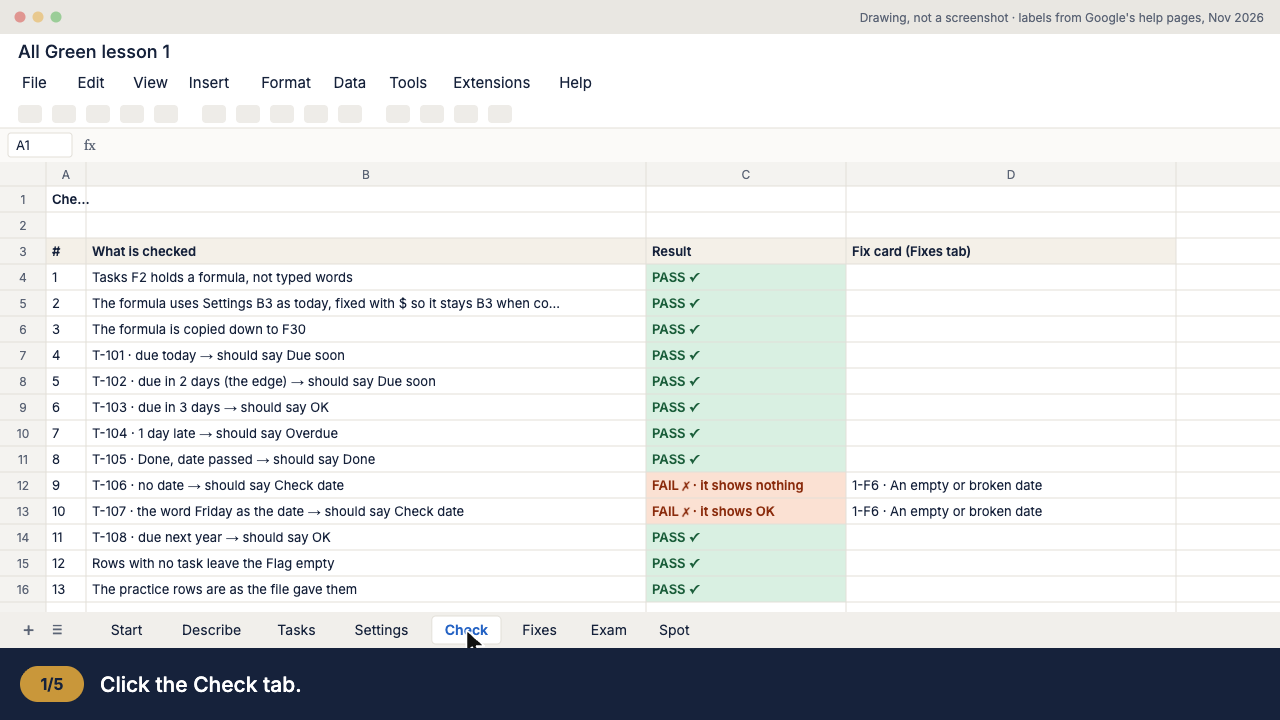
Open the Check tab. Each line checks one thing, in plain words, and says PASS ✓ or FAIL ✗:
- three lines about the formula itself: it is a formula; it uses Settings B3 as today, fixed with
$so it stays B3 when copied down; it is copied down to row 30; - one line for each practice row, with the label it should have;
- empty rows stay empty;
- the practice rows are still as the file gave them.
The total sits at the bottom, for example 13 of 13 PASS.
All 5 steps as text
- Click the Check tab.
- Scroll down to the total: 11 of 13 PASS. Red lines say FAIL; each names a fix card.
- Start with the first FAIL from the top: T-106 · no date → should say Check date.
- Its card is 1-F6: open the Fixes tab.
- Copy the text in the Paste this back column into the same AI chat, then paste the new formula over the old.
The checks know the right label for every practice row in advance. They look at what the formula does, not how it is written: any formula that gives the right labels passes, as long as it uses Settings B3 as today (line 2).
8. Fix
If a line says FAIL, start with the first FAIL from the top. Fixing it often fixes the lines below it.
- Read the code in column D, for example 1-F6 · An empty or broken date.
- Open the Fixes tab and find that code.
- Copy the text in the column Paste this back to your AI into the same chat.
- Paste the new formula over the old one in F2, copy it down again (step 6), and look at the Check tab.
Each fix card says what happened in plain words. For example:
1-F6 · An empty or broken date. Sheets treats an empty cell as 0 (the day 30 Dec 1899) when it compares dates, so an empty date looks long overdue. A word such as Friday is text, and comparing text with a date gives a wrong label or an error. Paste this back: Please check that the Due date is a real date with ISNUMBER before comparing it. If it is empty or not a number, the label is Check date.
If a cell shows an error such as #N/A or #VALUE!, use card E1: hover over the cell, and paste Google's message back to your AI.
8b. Fix practice: spot the bug, then fix it with your AI (about 3 minutes)
Your formula was all green at once? Most are: that is what the sheet's prompt is for. So here you practise the Fix step on a formula that is really wrong.
These three formulas were really written by an AI in our tests. One of them is wrong. Read them and guess which.
A
=IF(B2="","",IF(TRIM(LOWER(E2))="done","Done",IF(NOT(ISNUMBER(D2)),"Check date",IF(D2<Settings!$B$3,"Overdue",IF(D2<=Settings!$B$3+2,"Due soon","OK")))))B
=IF(E2="Done","Done",IF(D2="","",IF(D2<Settings!$B$3,"Overdue",IF(D2<=Settings!$B$3+2,"Due soon","OK"))))C
=IF(B2="","",IF(LOWER(TRIM(E2))="done","Done",IF(NOT(ISNUMBER(D2)),"Check date",IF(INT(D2)<INT(Settings!$B$3),"Overdue",IF(INT(D2)<=INT(Settings!$B$3)+2,"Due soon","OK")))))- Test your guess. On the Spot tab, paste one formula into F2, copy it down to F9, and read the Score in B11. Then try the next one.
What the Spot tab shows
A and C score 8 of 8. B scores 6 of 8. B leaves the task with no date empty, and it labels the word Friday as OK: a task you cannot see the date of is called fine. B answered a shorter request (step 11 shows it). We changed only its TODAY() to Settings!$B$3, so it can run on this tab.
- Now fix B with your own AI. Paste formula B into Spot F2 again and copy it down to F9 (6 of 8). Then send your AI this request: formula B, and the text of fix card 1-F6.
This Google Sheets formula labels the tasks on my tab Tasks. Column D is the Due date, column E the Status, and the cell Settings!$B$3 holds today: =IF(E2="Done","Done",IF(D2="","",IF(D2<Settings!$B$3,"Overdue",IF(D2<=Settings!$B$3+2,"Due soon","OK")))) Please check that the Due date is a real date with ISNUMBER before comparing it. If it is empty or not a number, the label is Check date. Give me the corrected formula on a single line.- Paste the formula it gives you into Spot F2, copy it down to F9, and read the Score: 8 of 8. The Start tab ticks step 8b.
That is the Fix step: a red line, its card, your AI, and green. In our tests this request fixed formula B in one reply in all 40 conversations: 20 of 20 with Claude Sonnet 5.5 and 20 of 20 with Claude Haiku 5.5, scored 8 of 8 on this Spot tab in our simulator.
9. Exam: rows your AI never saw
Passing the practice rows is good. It is not enough: the AI saw three of them in your prompt. The exam rows are new.
- Open the Exam tab. Click A5, hold Shift and click E14. Copy.
- Open the Tasks tab, click A2 and paste.
Two things change by themselves. Settings B3 moves today to Mon 14 Sep 2026, so a formula that typed in 10 March is caught. And the Check tab switches to the exam rows.

All 6 steps as text
- All green on the practice rows? Open the Exam tab.
- Click A5, hold Shift and click E14. Copy: Ctrl+C (Mac: Cmd+C).
- Open the Tasks tab and click A2.
- Paste: Ctrl+V (Mac: Cmd+V). New rows, and Settings B3 moves today to 14 Sep 2026.
- Your formula labels rows it never saw. Open the Check tab.
- 15 of 15 PASS: ALL GREEN. The banner shows your $5 code. Next: make it yours.
When all 15 lines pass, the Check tab says ALL GREEN and shows your code for $5 off the full course. The code works once the course is on sale; the course page says when.
To put the practice rows back: on the Exam tab, copy A20 to E29 (8 rows and 2 empty rows) and paste at Tasks A2.
10. Make it yours (before you go live)
Keep the exam rows in Tasks. Each change has its own check, so the right line turns red until your formula follows.
- Three days instead of two. Type
3in Describe B4. On the Check tab, E-02 turns red: it is due in 3 days, which is now Due soon. In your formula, find+2and change it to+3(click F2, edit in the formula bar, press Enter, then copy it down again: F2 to F30, Ctrl+D). The line turns green, and the Start tab ticks step 10. - Your own word. Type your own word in Describe B5, for example
Fix date. Two lines turn red: E-07 and E-08. In the formula, change"Check date"to"Fix date"and copy it down. They turn green. - A colour of your own (optional). The file already has one colour rule for each label. Change the colour of the rule for Due soon:

All 7 steps as text
- Make it yours: click any cell of the Tasks tab, then click Format.
- Click Conditional formatting. The panel lists the file's own rules, one per label.
- Click the rule for Due soon. Don't add a new one: the first true rule in the list sets the colour.
- The rule opens. Its formula stays as it is.
- Under Formatting style, pick a new fill colour.
- Click Done. The rule keeps its place in the list.
- Your eyes check this one, not the Check tab: every Due soon row has your colour.
Why change the file's rule instead of adding a new one? Google applies the rules in the order they are listed, and the first rule that is true sets the colour. A new rule for Due soon would sit below the file's own, so your colour would not show. (You can also drag a rule to the top of the list.) Your eyes check this one, not the Check tab.
11. Why it works, and when to use something else
The lowest rung. A formula like this is the safest kind of automation: it needs no permission, it cannot move or delete anything, and it updates by itself. (The exceptions are the IMPORT functions and IMAGE, which can reach the web once you click Allow access; step 5 tells you to refuse them.) Lessons 4 to 8 climb to scripts only when a formula cannot do the job.
The details are the job. We wrote a shorter request that leaves the details out, and sent it 20 times each to two AI models:
I have a Google Sheet with my tasks. Column D is the due date and column E is the status. Write a formula for column F that says Overdue, Due soon (due in the next 2 days), OK, or Done.
None of the 40 answers passed the checks. 36 of them labelled the word Friday as OK. The request never said what to do with a word in a date cell, so the AI guessed, and its guess hides a task. The prompt your sheet wrote names every one of those details. With it, all 40 answers passed (the record is below).
Pretend today. Date formulas fail at the edges: today, the last day of the window, the day after. A fixed date makes those edges testable, and the exam moves it to catch formulas that typed the date in.
When to use something else. If you need a message sent when a task is due, that is lesson 5 (a script). If you pay for Gemini in Google Sheets, it can write formulas inside your sheet too. Your checks still apply to whatever it writes.
12. Go live (the last step)
- In Settings B3, type
=TODAY()and press Enter. - On the Tasks tab, select A2 to E11 and press Delete. (The formulas in column F stay.)
- Type your own tasks. Each row gets its label as you type.
The Check tab now rests, and says why: its lines know only the lesson's rows. If you have more than 29 tasks, copy F30 further down; the colour rules already reach row 1000. To try the lesson's rows again later, import the lesson file into a new spreadsheet (then its time zone, as in step 2), so your own tasks stay as they are.
Words used in this lesson
| Word | Meaning |
|---|---|
| Tab | One sheet of the file. Their names are along the bottom. |
| Cell | One box of the grid, named by its column and row, such as F2. |
| Formula | What you type into a cell, starting with =, that works out the cell's value. |
| Formula bar | The long strip above the grid that starts with fx. It shows the formula of the cell you clicked. |
| Copy down | Copy a formula to the cells below it. Its cell names move with it (D2 becomes D3), except parts with $ signs. |
$ sign | Keeps part of a cell name fixed when you copy a formula: in Settings!$B$3, the $ before the 3 keeps it B3 in every row. |
| Practice rows | Rows with known right answers, used to check a formula. |
| Exam rows | New rows the AI never saw. A formula that only fits the examples fails here. |
Prompt card
Tested 2 Nov 2026 in our Google Sheets simulator (SheetSim):
20 fresh conversations each with Claude Sonnet 5.5 (claude-sonnet-5-5) and Claude Haiku 5.5 (claude-haiku-5-5),
through Claude Code's headless mode, with a plain one-line system prompt and no tools.
The prompt your sheet writes, all green on the first try, practice and exam rows: 20 of 20 and 20 of 20.
Step 8b, formula B with card 1-F6, fixed in one reply (8 of 8 on the Spot tab): 20 of 20 and 20 of 20.
The shorter request in step 11 (our own wording, details left out): 0 of 20 and 0 of 20.
36 of the 40 labelled the word Friday as OK.
Cards 1-F6 then 1-F5 pasted back after the shorter request (a separate batch of 20, Claude Sonnet only):
18 of 20 then gave the right label on every row, with TODAY() standing in for Settings B3. None of them used
Settings B3, so this workbook's Check tab would still show line 2 red: 0 of 20 all green here.
Also tried once in Gemini (gemini.google.com, free, signed in) on 17 Nov 2026, in Google Sheets: every flag line
green, on the practice and the exam rows.
Not tested: ChatGPT, Copilot, or the claude.ai chat itself. Your AI may answer differently.
Your sheet's checks are what protect you.Checked in Google Sheets on a free gmail.com Google account on 17 Nov 2026 (edition 1.0). Prompt tested: 2 Nov 2026, re-graded 17 Nov 2026. Edition 1.1. Not affiliated with Google. Google Sheets is a trademark of Google LLC. Claude is a trademark of Anthropic; Newel Labs is not affiliated with Anthropic.
How often does this prompt work?
We do not ask you to take the prompt on trust. On 2 Nov 2026 we sent it to two AI models, 20 fresh conversations each, and ran every answer through the workbook's own Check tab in our simulator:
| Claude Sonnet 5.5 | Claude Haiku 5.5 | |
|---|---|---|
| The prompt your sheet writes: all green first try | 20 of 20 | 20 of 20 |
| Step 8b, a wrong formula sent back with its fix card: fixed in one reply | 20 of 20 | 20 of 20 |
| A shorter request we wrote, leaving the details out (step 11 shows it) | 0 of 20 | 0 of 20 |
In the shorter request's answers, 36 of 40 labelled the word Friday in a date cell as OK.
We ran the models through Claude Code with a plain setup. On 17 Nov 2026 we also tried the prompt once in Gemini, free and signed in, in real Google Sheets: every flag line was green on the practice and the exam rows. We did not test ChatGPT, Copilot or the claude.ai chat itself, and your AI may answer differently. That is why every lesson's workbook checks the answer itself.
What comes next in Part 1: formulas the AI writes
- Lesson 2 · A tab that fills itself (about 15 minutes). A Done tab that lists every finished task, newest first, without moving or deleting a row. One formula with FILTER and SORT. Its checks keep working on your own rows after the lesson. In our simulator, a shorter request we wrote passed 0 of 40 times; the sheet's prompt, 40 of 40.
- Lesson 3 · Clean a messy export (about 30 minutes). Paste an export with name, email, date and amount columns into one tab; a second tab splits and capitalises names, fixes emails, turns text into real dates and numbers, and marks repeated customers. Its health lines then check your own exports. It teaches the one question only you can answer: which way round are your dates? With a shorter request we wrote, all 40 date formulas left that to the spreadsheet's locale.
Then Part 2 (scripts you run with a button, practice run first), Part 3 (automations that run on their own, each with an off switch) and Part 4 (your own chore).
All Green: the full course
- 9 lessons, about 5.3 hours of doing: 8 everyday automations and one of your own.
- 8 lesson workbooks that check your AI's work and a blank one for your own chore, fix cards, a course reader that works offline, and a PDF.
- Every update and every added lesson included.
- $29 once, tax included. Full refund within 30 days of purchase if it doesn't work for you — email support@newellabs.com.
- Your licence: for your own use, at home or at work. The workbooks, and the formulas and scripts you build in them, are yours to use and change for your own tasks and your own business. Please don't share, resell or re-upload the course files (lessons, PDF, reader, workbooks, cards).
- Finished lesson 1? Your workbook shows a code for $5 off when its exam is all green.
Sold by Polar, our merchant of record. No countdown, no "was" price.
Questions
Do I need to pay for an AI?
No, a free one is enough to try: whatever your AI writes, your sheet's checks grade it. We tested the prompts with Claude Sonnet 5.5 and Claude Haiku 5.5 through Claude Code, and on 17 Nov 2026 we tried lesson 1's prompt once in Gemini, free and signed in: its formula had every flag line green in Google Sheets. We did not test other chats.
Does my data go to the AI?
Only what you paste. The prompt the sheet writes holds invented practice rows, never your tasks. When you use the formula on your own tasks, it runs inside your Google Sheets, not in the AI.
Do I need Gemini or a paid Google plan?
No. The course uses no paid features: it is built for a free Google account, and lessons 1 to 3 were checked in Google Sheets on a free gmail.com Google account on 17 Nov 2026 (edition 1.0; the one check line that check found wrong is fixed in this edition and tested in our simulator). Lessons 4 to 9 were checked in Google Sheets on a free gmail.com Google account on 18 Nov 2026, in the United States locale: each menu item of lessons 4 to 8 with its Check tab, on the practice rows (in lessons 7 and 8 the exam rows too), a red run in each of lessons 4, 7 and 8, one run started by a one-off timer in each of lessons 6 and 8, and lesson 9's formula chore. Lesson 7 ran in PRACTICE mode only, lesson 8 never in LIVE mode, and no real form answer was sent. The time zone step and the corrected screen words came after that check, from what it saw; the time zone step is tested in our simulator. Gemini in Google Sheets needs an eligible paid plan; if you have it, the checks still apply to what it writes.
Can something break?
A formula like these only shows results, in its own cell or in empty cells beside it: it cannot move or delete anything. The exception is IMPORT and IMAGE formulas, which can send and receive data on the web after you click Allow access. Our prompts ask for none; if your AI's formula has one, don't allow access, and ask for a formula without it. Scripts start in lesson 4, and each one has a practice mode that only lists what it would do.
What may I do with the files?
Lesson 1 is free to use, at home or at work, and free to share unchanged with a link to newellabs.com/learn/all-green/; it is not for resale. The paid course is for your own use, at home or at work: the formulas and scripts you build are yours, but please don't share or resell the course files.
Does it work in Excel?
The lessons and their screens are for Google Sheets. Lesson 1's reference formula uses only functions that Excel also has (not tried in Excel), but an AI's answer may use functions only Google Sheets has, and this course does not teach Excel.
Who made this?
Claude, an AI model made by Anthropic, wrote and built the course for Newel Labs. Newel Labs is not affiliated with Google or Anthropic. Google Sheets is a trademark of Google LLC, and Claude is a trademark of Anthropic.